

Deriving the Spring Mass System Differential Equation from First Principles
Mechanical vibration analysis begins by understanding how restoring forces interact with accelerating bodies. When studying The Science of Springs: How They Work, the core principle governing mechanical deflection is Hooke’s law. This physical law states that the restoring force exerted by an elastic spring is directly proportional to its displacement from equilibrium, acting in the opposite direction.
When calculating a spring constant using Hooke’s law, the relationship is expressed as:
F_spring = -k * x
In this expression, k represents the spring constant, and x denotes displacement. When an external mass attaches to this elastic member, Newton’s second law governs the dynamic behavior:
F_net = m * a = m * x”
By accounting for all acting forces, including internal restoring forces, viscous resistance, and external driving functions, engineers establish the fundamental equations of motion.
Setting Up Coordinate Frames and Static Deflection
Consider a mass suspended vertically from a rigid ceiling by an elastic extension spring. Before any dynamic motion begins, the mass stretches the spring downward by a static distance, denoted as L or s_0, until it reaches a resting state known as the static equilibrium position.
When calculating spring deflection at rest, the downward gravitational force balances the upward spring tension:
m * g = k * L
By establishing the origin of our coordinate system (x = 0) exactly at this static equilibrium position, downward displacement is defined as positive (+x) and upward displacement as negative (-x). When the mass moves dynamically to an arbitrary position x(t), the total elongation of the spring becomes (L + x). The total restoring force exerted by the spring is:
F_spring = -k * (L + x)
Formulating the Undamped Spring Mass System Differential Equation
Summing all vertical forces acting on the dynamic mass yields:
F_net = m * g – k * (L + x)
Expanding this equation reveals an elegant mathematical cancellation:
F_net = m * g – k * L – k * x
Because the system was configured around static equilibrium, m * g equals k * L. These two terms subtract to zero, leaving:
F_net = -k * x
Equating this net force to the inertial acceleration term from Newton’s second law produces the homogeneous second-order ordinary differential equation:
m * x” = -k * x
Rearranging this expression into standard form yields:
m * x” + k * x = 0
Dividing through by mass gives the clean harmonic oscillator relationship:
x” + (k / m) * x = 0
Solving Free Undamped Vibrations and Simple Harmonic Motion
To determine the dynamic position of the mass over time, we solve the homogeneous linear differential equation. Assuming a general solution of exponential form x(t) = e^(r * t), substituting its derivatives into the governing equation produces the characteristic equation:
m * r^2 + k = 0
Solving for the roots yields:
r^2 = -k / m
r = ± i * sqrt(k / m)
Because the roots are purely imaginary complex conjugates, Euler’s formula translates the general solution into a linear combination of trigonometric functions:
x(t) = c1 * cos(omega0 * t) + c2 * sin(omega0 * t)
The units of dynamic stiffness and mass balance each other in the argument of these trigonometric functions, as detailed when evaluating the spring constant dimensional formula 101. The unknown constants c1 and c2 are determined using initial value problem boundary conditions, where initial position is x(0) = x0 and initial velocity is x'(0) = v0:
c1 = x0
c2 = v0 / omega_0
Calculating Natural Frequency, Period, and Amplitude-Phase Form
The angular natural frequency of the undamped system is defined as:
omega_0 = sqrt(k / m)
This frequency is measured in radians per second. The corresponding natural cyclic frequency and oscillation period are:
f0 = omega0 / (2 * pi)
T = (2 * pi) / omega_0 = 2 * pi * sqrt(m / k)
While a combination of sine and cosine terms fully describes the motion, expressing the displacement as a single sinusoid provides clear physical insight into amplitude and phase:
x(t) = A * cos(omega_0 * t – phi)
Here, the total physical amplitude A and phase angle phi are:
A = sqrt(c1^2 + c2^2) = sqrt(x0^2 + (v0 / omega_0)^2)
phi = arctan(c2 / c1)
When calculating the phase shift phi, engineers must verify the trigonometric quadrant by matching the individual algebraic signs of c1 and c2.
Analyzing Damped Systems: Overdamped, Critically Damped, and Underdamped Motion
Real-world mechanical systems experience energy dissipation due to fluid resistance, material friction, or mechanical dashpots. Viscous damping produces an opposing force proportional to velocity:
F_damping = -b * x’
Adding this resistance to Newton’s force balance yields the damped equation of motion:
m * x” + b * x’ + k * x = 0
The corresponding characteristic auxiliary equation is:
m * r^2 + b * r + k = 0
Using the quadratic formula, the characteristic roots are:
r = (-b ± sqrt(b^2 – 4 * m * k)) / (2 * m)
The behavior of the mechanical system depends entirely on the discriminant (b^2 – 4 * m * k).
| Damping Regime | Mathematical Condition | Root Characteristics | Physical Motion Behavior |
|---|---|---|---|
| Overdamped | b^2 > 4 * m * k | Two distinct real negative roots | Slow, non-oscillatory return to equilibrium |
| Critically Damped | b^2 = 4 * m * k | Repeated real negative root | Fastest non-oscillatory settling to equilibrium |
| Underdamped | b^2 < 4 * m * k | Complex conjugate roots with negative real parts | Decaying harmonic oscillations within an exponential envelope |
Evaluating the Three Damping Regimes

In an overdamped system, the viscous resistance dominates elastic stiffness. The characteristic roots r1 and r2 are distinct, negative, real numbers:
x(t) = c1 * e^(r1 * t) + c2 * e^(r2 * t)
The mass returns to equilibrium without oscillating. High resistance can make this return sluggish.
Critical damping represents the boundary between oscillatory motion and pure exponential decay. The critical damping coefficient is:
b_cr = 2 * sqrt(m * k)
When damping matches this value, the characteristic equation yields repeated real roots, producing the solution:
x(t) = (c1 + c2 * t) * e^(-(b / (2 * m)) * t)
Critical damping returns the mass to equilibrium in the shortest possible time without overshoot. In physical engineering, systems are rarely perfectly critically damped because maintaining exact theoretical equality is difficult in production environments.
In an underdamped system, elastic restoring forces exceed viscous dissipation. The characteristic roots are complex conjugates:
r = alpha ± i * omega_d
alpha = -b / (2 * m)
omegad = sqrt(4 * m * k – b^2) / (2 * m) = omega0 * sqrt(1 – zeta^2)
Here, zeta = b / (2 * sqrt(m * k)) represents the damping ratio. The resulting displacement equation is:
x(t) = e^(alpha * t) * (c1 * cos(omegad * t) + c2 * sin(omegad * t))
The mass oscillates with a reduced damped angular frequency omega_d while its amplitude decays within an exponential envelope defined by e^(alpha * t).
Forced Oscillations, Resonance, and Dynamic System Analogies
When external periodic forces act upon a mechanical assembly, such as an engine vibration or cyclic road input, the governing differential equation becomes nonhomogeneous:
m * x” + b * x’ + k * x = F_0 * cos(omega * t)
Here, F_0 represents the excitation magnitude, and omega represents the driving frequency. The general solution combines the complementary homogeneous solution and the particular integral:
x(t) = xtransient(t) + xsteady-state(t)
The transient response xtransient(t) is governed by the system’s natural damping characteristics and decays exponentially to zero over time. The steady-state response xsteady-state(t) persists indefinitely, driven by the external excitation:
x_steady-state(t) = X * cos(omega * t – theta)
When evaluating spring stiffness during cyclic loads, knowing how to calculate spring rate for compression springs ensures the steady-state mechanical deflection remains within safe operating limits.
Avoiding Mechanical Resonance in Forced Vibrations
Mechanical resonance occurs when the external forcing frequency omega approaches the system natural frequency omega0. In an undamped system where omega equals omega0, the particular solution takes the form:
xp(t) = (F0 / (2 * m * omega0)) * t * sin(omega0 * t)
Because this displacement grows proportionally with time t, oscillation amplitudes escalate rapidly, potentially leading to catastrophic mechanical fatigue, component failure, or structural collapse. A well-known historical example of destructive aerodynamic resonance is the collapse of the Tacoma Narrows Bridge in 1940.
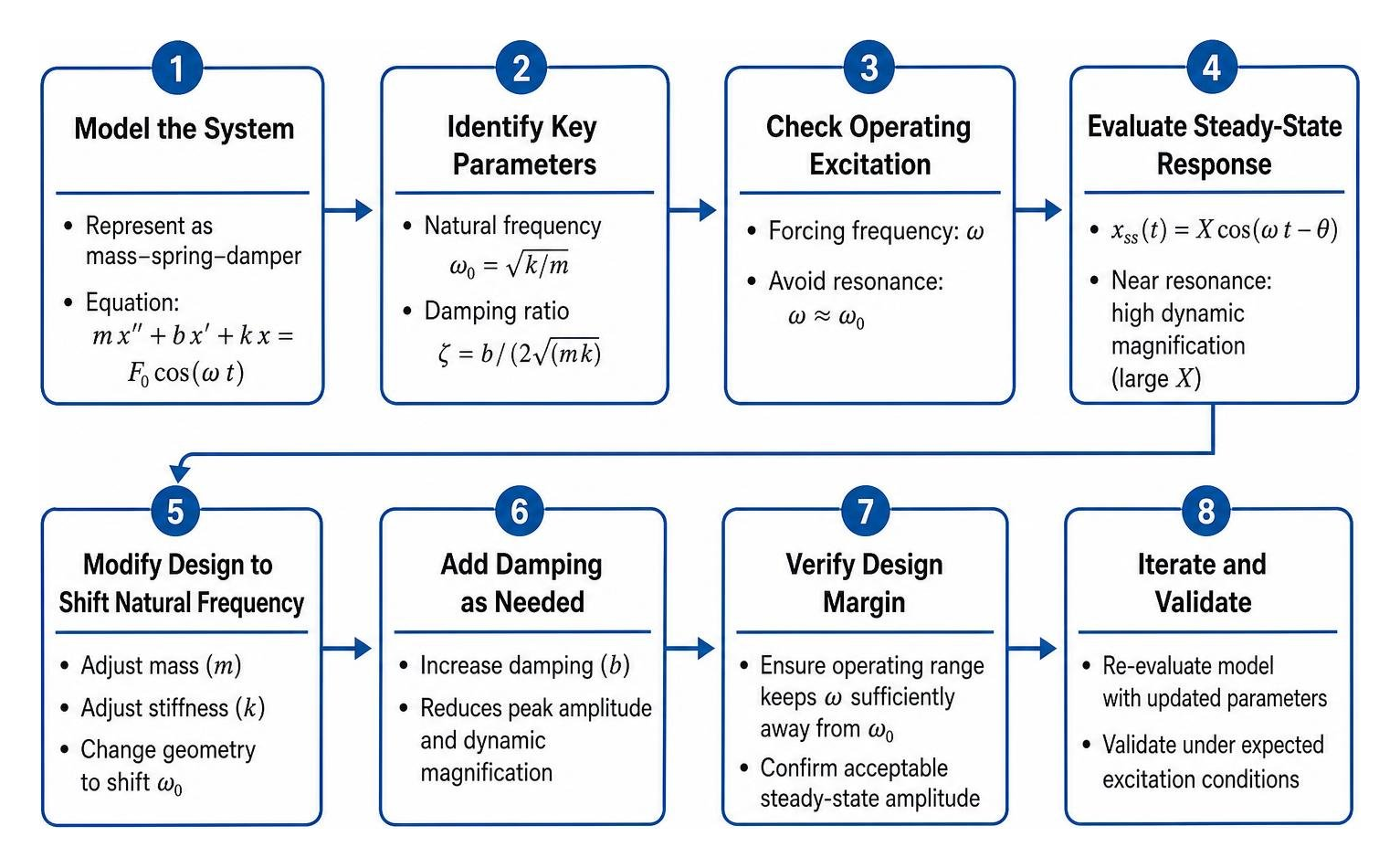
In real-world damped systems, damping limits the peak amplitude, but high dynamic magnification can still cause severe wear. Engineers prevent resonance by altering component mass, modifying spring geometries, or incorporating tuned viscous dampers to shift natural frequencies away from operating excitation ranges.
Solving the Forced Damped Spring Mass System Differential Equation with RLC Circuit Analogies
The mathematical framework used in mechanical vibrations maps directly to electrical circuit analysis. A series RLC circuit containing an inductor (L), resistor (R), capacitor (C), and voltage source E(t) obeys Kirchhoff’s voltage law:
L * q” + R * q’ + (1 / C) * q = E(t)
Here, q represents electrical charge, q’ is electrical current, and q” is the rate of current change.
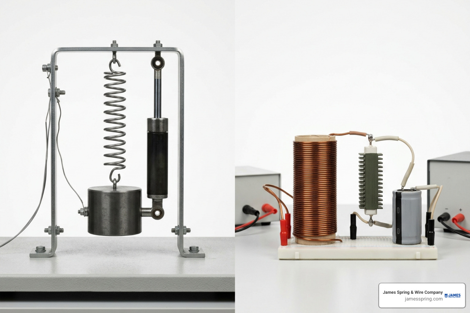
The analogies between these two physical systems are direct:
- Mass (m) corresponds to Inductance (L), representing inertial resistance to changes in motion or current.
- Damping coefficient (b) corresponds to Resistance (R), representing energy dissipation.
- Spring constant (k) corresponds to Elastance or reciprocal Capacitance (1 / C), representing potential energy storage.
- Displacement (x) corresponds to Electric Charge (q).
- Velocity (x’) corresponds to Electric Current (i = dq/dt).
- Applied Force f(t) corresponds to Applied Voltage E(t).
Because the underlying differential equations are identical, electrical filter design methods, tuning techniques, and damping calculations transfer directly into mechanical engineering analysis.
Frequently Asked Questions about Spring Mass Differential Equations
Why does gravity cancel out in vertical spring mass differential equations?
Gravity cancels out because the coordinate origin (x = 0) is placed at the static equilibrium position. When the mass is suspended at rest, it causes a static deflection L where the downward force of gravity (m * g) exactly equals the upward elastic tension (k * L). When dynamic motion begins, the total spring force is -k * (L + x). Expanding this into -k * L – k * x cancels out the gravitational term m * g, leaving only the dynamic restoring force -k * x.
What is the physical significance of critical damping in engineering design?
Critical damping represents the exact threshold where a displaced mass returns to its equilibrium position in the minimum possible time without oscillating. In mechanical applications like automotive shock absorbers, firearm recoil buffers, and precision sensor scales, critical damping eliminates unwanted vibrations while preventing sluggish settling behavior.
How do transient and steady-state responses differ in forced spring systems?
The transient response is the portion of the solution derived from the homogeneous differential equation. Because of viscous damping, this response decays exponentially to zero shortly after excitation begins. The steady-state response is the particular solution driven by the continuous external force. It dictates long-term behavior, maintaining constant amplitude and oscillating at the driving frequency as long as the external excitation persists.
Conclusion
Deriving and solving differential equations for spring-mass systems gives engineers the mathematical tools needed to predict dynamic stability, vibration settling, and resonance risks. Translating physical forces into second-order equations helps teams optimize spring stiffness, damping ratios, and mass distributions across complex mechanical assemblies.
When your application requires high-performance components manufactured to tight tolerances, working with an experienced OEM partner is essential. James Spring & Wire Company designs and manufactures standard and custom compression springs, extension springs, torsion springs, and precision wire forms. Backed by over 60 years of in-house expertise and ISO 9001 certified quality systems, our team delivers consistent components for demanding automotive, medical, and industrial applications.
To discuss your mechanical specifications or get manufacturing support for your next dynamic assembly, request a quote for custom precision springs today.